
Le MOPITT à vingt-cinq ans : un quart de siècle de science
– Par Paul Jeffery –
Le satellite Terra de la National Aeronautics and Space Administration (NASA), satellite phare du programme Earth Observing System (EOS) de la NASA,
– Par Paul Jeffery –
Le satellite Terra de la National Aeronautics and Space Administration (NASA), satellite phare du programme Earth Observing System (EOS) de la NASA,

– Par Stephanie Cleland –
Les changements climatiques entraînent une hausse des températures et une modification des conditions météorologiques à l’échelle du Canada et dans le monde.

– Par Douglas W.R. Wallace –
La mise hors service soudaine, mais pas inattendue en janvier 2022, du navire de recherche de la Garde côtière canadienne NGCC Hudson,

– Par David Allan et Richard Allan –
De nombreuses personnes qui s’intéressent à l’océanographie ont déjà rencontré le blob froid ou « trou de réchauffement »,

Les présentations de résumés sont maintenant acceptées!

– Par Muriel Dunn et Martin Ludvigsen –
Au cours de la première semaine de juin 2024, le groupe de terrain (trois robots océaniques et trois ingénieurs) s’est rendu à la magnifique station de Mausund pour une semaine de travail sur le terrain.

– Par Emma Harrison –
« À cette date en 1988, je traversais le lac Melville en motoneige. J’espère me tromper complètement, mais tout indique que nous nous dirigeons vers une autre saison tardive. »
18 novembre 2023 — Derrick Pottle, observateur Nunatsiavut des glaces de mer pour Rigolet

– Par Yeechian Low –
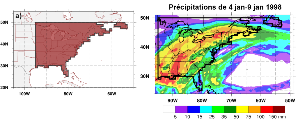

– Par Paul Joe, Ronald E. Stewart et Sudesh Boodoo –
Une analyse radar de la tempête de grêle du 13 juin 2020 à Calgary est présentée.