Le réchauffement climatique est-il à l’origine de l’atlantification de la mer de Barents, de l’effondrement des courants de l’Atlantique Nord, ou d’aucun des deux?

– Par Knut Seip et Hui Wang –

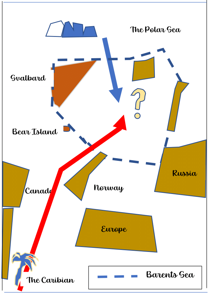
Cette étude porte sur la mer de Barents et deux courants de l’Atlantique Nord, la circulation méridienne de retournement de l’Atlantique (AMOC) et l’oscillation atlantique multidécennale (OAM), et sur ce qui se passe lorsque les courants de l’Atlantique Nord atteignent la mer de Barents.

L’OAM et l’AMOC sont deux courants qui ont un impact important sur le climat de l’hémisphère nord. Les courants chauds, comme le Gulf Stream, qui font partie de l’AMOC, viennent des Caraïbes et rencontrent l’eau froide de la mer de Barents. Trois effets majeurs de l’OAM et de l’AMOC sur la mer de Barents sont suggérés en raison du réchauffement climatique. Tout d’abord, la mer de Barents sera atlantifiée (Barton et coll. 2018) et l’écosystème de la mer de Barents sera similaire à celui de l’Atlantique Nord (Ingvaldsen et coll. 2021). Deuxièmement, l’eau froide et alimentée par la glace de la mer de Barents se déplace dans l’Atlantique Nord et modifie considérablement les courants atlantiques. Dans un scénario extrême, l’AMOC s’effondrera (Ditlevsen et Ditlevsen 2023) et une baisse soudaine et importante de la température dans le nord de l’Europe et des États-Unis peut survenir. Le troisième scénario est qu’il n’y a pas d’effet de la mer de Barents sur l’AMOC et l’OAM (Li et coll. 2021) ou vice versa.

Étant donné que les courants océaniques présentent une variabilité (très probablement avec des pseudo-cycles), nous pouvons supposer qu’un pic dans la variable causale se produira avant un pic dans la variable de l’effet. Par conséquent, si l’AMOC atteint un pic avant le pic des cycles dans la mer de Barents, cela veut dire que les températures des eaux de l’Atlantique ont un impact sur la température des eaux de la mer de Barents. Si l’AMOC atteint son maximum après les pics de courant dans la mer de Barents, alors c’est la mer de Barents qui influe sur les eaux de l’Atlantique Nord et l’AMOC.

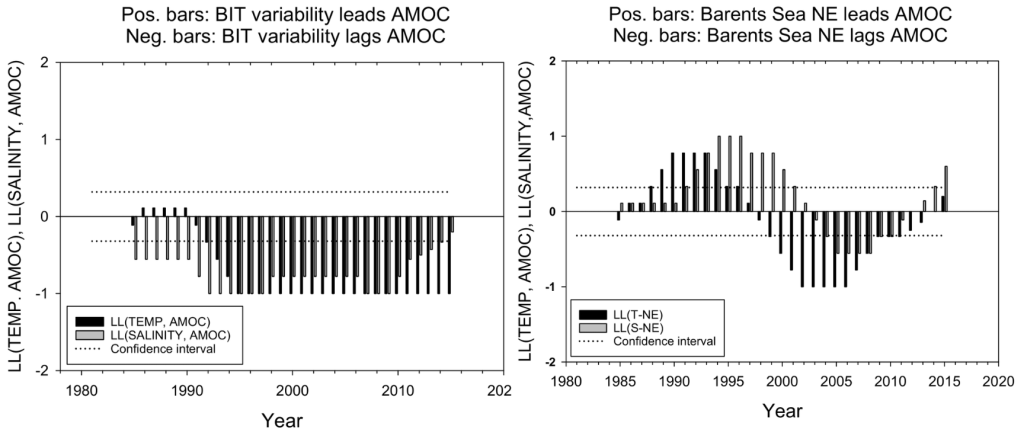
Pour utiliser les données sur les relations entre les courants océaniques, il faut une méthode qui quantifie les relations entre les courants océaniques sur des périodes de temps très courtes. L’astuce pour y parvenir est expliquée dans la section sur la méthode ci-dessous. Pour vérifier si le résultat est significatif, nous procédons comme d’habitude. Nous comparons la persistance d’une relation LL à celle de deux séries stochastiques. Plus une relation de premier plan est persistante, plus nous sommes confiants dans son effet causal. Et c’est encore mieux si les périodes du cycle changent en durée (les séries sont non stationnaires), et que les deux séries montrent toujours des relations LL persistantes. Pour montrer les relations LL résultantes entre deux séries temporelles, nous utilisons un graphique avec des barres qui sont soit positives (la première série précède la seconde), soit négatives (la seconde série précède la première) dans la figure 2.

Nous examinons deux entrées pour l’AMOC dans la mer de Barents. Les pics de la série AMOC ont précédé les pics des courants observés dans le fossé de l’île Bear (BIT, l’un des bras de mer) de 1991 à 2014, soit 23 ans (figure 2a). Cependant, dans l’entrée au nord-est de la mer de Barents (BSNE), il y a d’abord une courte période de six ans où les courants de la mer de Barents devancent l’AMOC, puis une seconde courte période de huit ans où l’AMOC devance les courants de la mer de Barents (figure 2b).

Les séries temporelles du transport de chaleur et de salinité entre les eaux de l’Atlantique Nord et la mer de Barents sont fondées sur des observations. Nos résultats et l’interprétation des données donnent à penser que la chaleur et le sel sont transportés dans les deux sens, et avec un rythme différent dans les deux régions où l’AMOC rencontre la mer de Barents.

Si nous supposons que les flux d’eau à travers les deux entrées sont de taille similaire, c’est le flux entrant au BIT, à savoir l’eau transportée par l’AMOC et l’OAM, qui domine les eaux de la mer de Barents au cours de la période 1971-2014. L’entrée par le BIT peut avoir une section transversale plus grande que l’entrée à la BSNE (Barton et coll. 2018).

Nous avons aussi obtenu un deuxième résultat. Nous avons observé que les variations de température dans les eaux de surface de la mer de Barents précèdent toujours les variations de température dans les eaux intermédiaires, donnant à penser que les variations de chaleur dans l’atmosphère sont transportées vers les eaux de la mer de Barents (graphiques non montrés).

Notre conclusion est que les températures dans la mer de Barents sont influencées par les variations de température dans l’atmosphère et par les variations de température dans les eaux de l’Atlantique Nord (l’AMOC et l’OAM) jusqu’en 2000 environ. De plus, les variations de température dans la mer de Barents sont attribuables à la fonte des glaces et aux changements d’albédo qui l’accompagnent. Après 2018 environ, le réchauffement climatique pourrait jouer un rôle de plus en plus important dans le système de station océanique de l’Atlantique Nord de la mer de Barents.

– By Knut L. Seip and Hui Wang –

This study is about the Barents Sea and two North Atlantic currents, the Atlantic meridional overturning circulation (AMOC) and the Atlantic multidecadal oscillation (AMO) and what happens when the North Atlantic currents reach the Barents Sea.

Why are the AMO and the AMOC important?

The AMO and the AMOC are two currents that are shown to strongly impact the climate on the Northern Hemisphere. The trajectory for the AMOC is sketched in Figure 1. Warm currents, like the Gulf Stream, which are part of the AMOC, are coming from the Caribbean and meet cold water in the Barents Sea. Three major effects from AMO and AMOC on the Barents Sea are suggested because of global warming. First, the Barents Sea will be Atlantificatied (Barton et al. 2018) and the ecosystem of the Barents Sea will be similar to that of the North Atlantic (Ingvaldsen et al. 2021). Second, the cold and ice fed water in the Barents Sea moves into the North Atlantic and changes the Atlantic currents dramatically. In an extreme scenario, the AMOC will collapse (Ditlevsen and Ditlevsen 2023) and a sudden and severe decrease in temperature across northern Europe and the United States can occur.  The third scenario is that there is no effect from the Barents Sea on the AMOC and AMO (Li et al. 2021) or vice versa.

How to get closer to the answer

Since ocean currents show variability (most probably with pseudo cycles), we can assume that a peak in the causal variable would occur before a peak in the effect variable. Therefore, if AMOC peaks before cycles peak in the Barents Sea, we interpret this as meaning that the temperatures in the Atlantic waters impact the temperature in the waters of the Barents Sea. If AMOC peaks after the current peaks in the Barents Sea, then it is the Barents Sea that affects the North Atlantic waters and the AMOC.

The real story is a little bit more complicated. The AMOC is measured in cubic meters per second (Sv), the AMO in ^oC, and salinity also plays a role. However, here we focus on the temperature part and on AMOC.

To use the information on lead and lag (LL) relations between ocean currents, you need a method that quantifies LL relations over very short time spans. The trick to do that is explained in the method section below. To test if the result is significant, we do as one always does. We compare the persistence of an LL relation to that of two stochastic series. The more persistent a leading relation is, the more confident we are in its causal effect. And it is even better if the cycle periods change in duration (the series are non-stationary), and the two series still show persistent LL relations. To show the resulting LL relations between two time series, we use a graph with bars that are either positive (the first series leads the second) or negative (the second series leads the first) in Figure 2.

We got two results

We examine two inlets for the AMOC to the Barents Sea. The peaks in the AMOC series came before the peaks in the currents that was observed in the Bear Island trough (BIT, one of the inlets) from the year 1991 to 2014, that is 23 years, Figure 2a. However, in the inlet at the Barents Sea northeast (BSNE), there is first a short period of 6 years where the Barents Sea currents lead the AMOC, but then a second short period of 8 years where the AMOC leads the Barents Sea currents, Figure 2b.

Time series for heat and salinity transport between the North Atlantic waters and the Barents Sea are based on observations. Our results and interpretation of the data suggest that heat and salt are transported both ways, and with different timing at the two regions where the AMOC meets the Barents Sea.

If we assume that the water flows through the two inlets are similar in size, then it is the inflow at the BIT, that is, the water carried with the AMOC and the AMO that dominates the waters in the Barents Sea during the period 1971 to 2014. The inlet through the BIT may have a larger cross section than the inlet at the BSNE (Barton et al. 2018).

We also obtained a second result. We found that temperature variations in the surface water of the Barents Sea always lead the temperature variations in the intermediate water, suggesting that heat variations in the atmosphere are transported to the Barents Sea waters (graphs not shown).

Our conclusion is that temperatures in the Barents Sea are influenced by temperature variations in the atmosphere and by temperature variations in the North Atlantic waters (the AMOC and the AMO) until about 2000. In addition, temperature variations within the Barents Sea are caused by ice melting and accompanying changes in albedo. After about 2018 global warming may play an increasingly important role in the Barents Sea-North Atlantic Ocean system.

There are four caveats in our results. i) The assumption that the flow through the BIT is larger or of about equal size to the flow through the BSNE may not be correct, and there are more gateways to the Barents Sea than those two studied here. ii) The study period was only 48 years, and ocean currents may change directions after that time (Seip et al. 2023). iii) Global warming may alter ocean flow patterns in the Barents Sea and in the North Atlantic. In particular, the return flow of cold-water at large depths may change characteristics. iv) Last, the atmosphere-ocean exchange of heat may change with global warming and global cooling (Li et al. 2023).

The method trick

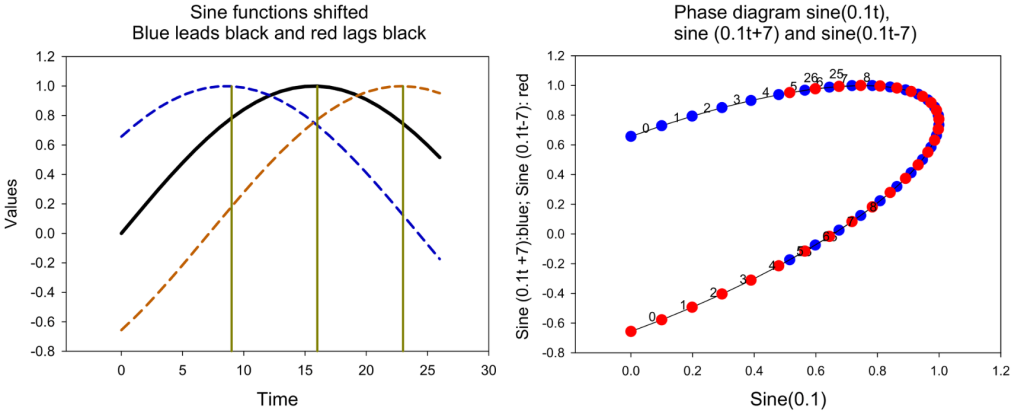
The trick to distinguish lead-lag patterns is to depict the potential causal and effect series in a phase plot. In such a plot, we can determine the lead-lag pattern based on three paired consecutive observations (and not only for the peaks or troughs). Figure 3 shows that if one time series peaks before another (blue and black in Figure 3, black on the x-axis), then the trajectories rotate clockwise. If one time series peaks after another (black and red, black on the x-axis), then the trajectories rotate counterclockwise.

Although it may be easy to see the relation between series in a phase diagram, the equation that calculates rotational directions in the phase diagram could be difficult to write out. For readers that are interested we would be glad to provide a one-page spread sheet (Excel book) with the appropriate calculations. Then, to use the method, just paste the time series into two columns in the spread sheet.

Knut L. Seip is professor emeritus at Oslo Metropolitan University.  He has recently been working on aquatic and economic problems using a high-resolution lead-lag (cause before effect) methodology to disentangle causal variable in observed time series.

Hui Wang is a meteorologist from the Climate Prediction Center of the U.S. National Oceanic and Atmospheric Administration. His research interests are climate variability, climate modelling and prediction.

References

Barton, B. I., Y. D. Lenn and C. Lique (2018). “Observed Atlantification of the Barents Sea Causes the Polar Front to Limit the Expansion of Winter Sea Ice.” Journal of Physical Oceanography 48(8): 1849-1866.

Ditlevsen, P. and S. Ditlevsen (2023). “Warning of a forthcoming collapse of the Atlantic meridional overturning circulation.” Nature Communications 14(1).

Ingvaldsen, R. B., K. M. Assmann, R. Primicerio, M. Fossheim, I. V. Polyakov and A. V. Dolgov (2021). “Physical manifestations and ecological implications of Arctic Atlantification.” Nature Reviews Earth & Environment 2(12): 874-889.

Li, F., M. S. Lozier, S. Bacon, A. S. Bower, S. A. Cunningham, M. F. de Jong, B. DeYoung, N. Fraser, N. Fried, G. Han, N. P. Holliday, J. Holte, L. Houpert, M. E. Inall, W. E. Johns, S. Jones, C. Johnson, J. Karstensen, I. A. Le Bras, P. Lherminier, X. Lin, H. Mercier, M. Oltmanns, A. Pacini, T. Petit, R. S. Pickart, D. Rayner, F. Straneo, V. Thierry, M. Visbeck, I. Yashayaev and C. Zhou (2021). “Subpolar North Atlantic western boundary density anomalies and the Meridional Overturning Circulation.” Nature Communications 12(1).

Li, H., J. Richter, H, A. Hu, G. A. Meehl and D. MacMartin (2023). “Responses in the subpolar North Atlantic in two climate model sensitivity experiments with increased stratospheric aerosols.” Journal of Climate: 1-31.

Seip, K. L., Ø. Grøn and H. Wang (2023). “Global lead‑lag changes between climate variability series coincide with major phase shifts in the Pacific decadal oscillation.” Theoretical and Applied climatology.