Exploration précoce de la stratosphère des hautes latitudes – Partie II : Découverte du courant-jet de la nuit polaire

– Par Kevin Hamilton–

Comme le montre la première partie, au milieu des années 1930, la climatologie de base de la température stratosphérique jusqu’à ~30 km était comprise. Dans la basse stratosphère, on a constaté un fort cycle saisonnier de la température aux hautes latitudes, notamment avec un pôle d’hiver froid compatible avec un cisaillement vertical moyen d’ouest et un vortex d’ouest circumpolaire.

Dans sa conférence commémorative Symons de 1935, le mathématicien et physicien anglais Francis Whipple a noté une conséquence de la nouvelle compréhension de la climatologie de la température, à savoir que la différence de pression horizontale à 20 km entre « l’Angleterre » et la « Laponie » s’inverse en été et en hiver, ce qui permet de s’attendre à un flux géostrophique moyen dans la bande de latitude ~50^o-70^oN à ce niveau, qui est de l’est en été et de l’ouest en hiver. Il a noté que cela correspondait aux observations faites pendant la Première Guerre mondiale, selon lesquelles les bruits de la bataille en France n’étaient entendus loin à l’ouest, près de Londres, qu’en été. Une telle propagation à longue distance donne lieu à des fronts d’ondes sonores qui se sont réfractés vers le haut dans la stratosphère, puis redescendent de la stratosphère vers le sol; leur propagation est sensible à la température et au vent stratosphériques.

Au cours du quart de siècle suivant, cette idée précoce sera affinée en une image détaillée de la structure typique du vent dans la stratosphère tout au long du cycle annuel. Cet article est consacré à l’examen des progrès réalisés dans l’observation du champ de vent stratosphérique, en  mettant l’accent sur la découverte du courant-jet polaire nocturne.

– By Kevin Hamilton –

Introduction

As shown in Part I, by the mid-1930’s the basic climatology of stratospheric temperature up to ~30 km was understood. In the lower stratosphere a strong seasonal cycle of temperature at high latitudes was found, notably with a cold winter pole consistent with a westerly mean vertical shear and a circumpolar westerly vortex.

In his 1935 Symons Memorial Lecture English mathematician and physicist Francis Whipple noted a consequence of the newly found understanding of the temperature climatology, specifically that the horizontal pressure difference at 20 km between “England” and “Lapland” reversed in summer and winter, leading to expectation of mean geostrophic flow in the latitude band ~50o-70oN at this level that is easterly in summer and westerly in winter. He noted that this was consistent with observations during World War I that the sounds of battle in France were heard far to the west, near London, only in summer. Such long-distance propagation involves sound wave fronts that have refracted upward into the stratosphere and then back downward from the stratosphere to the ground; their propagation is sensitive to the stratospheric temperature and wind.

Over the next quarter-century this early insight would be refined into a detailed picture of the typical wind structure in the stratosphere through the annual cycle. This paper is devoted to a review of this progress in observing the stratospheric wind field, with a focus on the discovery of the polar night jet stream.

Very Early Direct Wind Observations in the Stratosphere

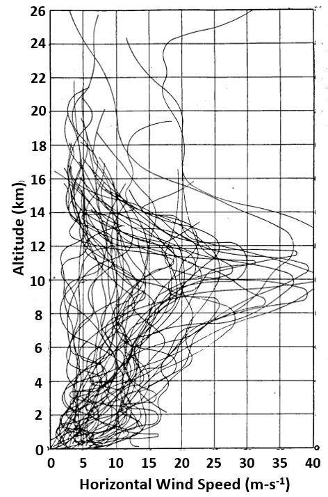
Before radio tracking techniques were developed, measurements of the wind high above the ground depended on optical theodolite tracking of balloons, and this only rarely allowed winds to be observed up to stratospheric levels. The English meteorologist Gordon Dobson (1920) seems to have been the first to systematically investigate the stratospheric winds. Dobson analyzed a total of 70 soundings from several European stations during the period 1904-1912 that featured (i) recovery of the registering sonde (and hence observation of the temperature profile and the location of the tropopause), and (ii) penetration above the tropopause, and (iii) theodolite tracking of the winds into the stratosphere. Dobson’s result is reproduced here as Figure 1. Only 4 of these profiles extended above 22 km and almost all the profiles display peak winds near the tropopause and a rapid drop off with height in the first few km of the stratosphere.

Jet Streams

Today we are familiar with the idea that the large-scale atmospheric circulation typically features intense narrow currents or “jet streams” primarily aligned in the zonal direction. The recognition of the existence and significance of various jet streams in the atmosphere emerged over time. The atmospheric aerosol after the 1883 Krakatoa eruption in Indonesia was tracked as it circled the earth in a narrow region around the equator. An amateur scientist from Hawaii named Sereno Bishop within a year had coined the term “smoke stream” for this phenomenon. Today we know that this jet-like wind is characteristic of the equatorial stratosphere and Bishop arguably deserves credit for discovering the first “jet stream” in the atmosphere.

In the early decades of the 20th century there were scattered reports of strong midlatitude winds near tropopause levels measured by pilot balloons. Particularly notable were pilot balloon observations taken near Tokyo (36^oN) by the Japanese meteorologist Wasuburo Ooishi in the early and mid-1920’s. He found that the winds near 10 km in winter were typically very strong westerlies, with one notable sounding in December 1924 showing a westerly wind of more than 70 m-s^-1 at 9 km.

In the 1930’s knowledge of the winds in the upper troposphere began accumulating from observations during high altitude aircraft flights. In 1934 and 1935 the pioneer high-altitude aviator (and inventor of the pressurized flight suit) Wiley Post experienced wind speeds in excess of about 50 m-s^-1 when flying in the upper troposphere over the US. In 1939 the German meteorologist Seilkopf noted strong winds measured around midtroposphere by aircraft in Europe and coined the term strahlströmmung (“jet flow”). In World War II the US military were surprised by the strong headwinds encountered by B-29 bombers as they flew high altitude missions to Japan. It appears that Rossby, then at the University of Chicago, originated the English language term “jet stream” for these very strong winds. During WWII Herbert Riehl, later a leader in the study of tropical meteorology, was a graduate student at the University of Chicago and a meteorology instructor for the US military. He later recalled that

“… we were most impressed by the news that B-29s sent westward to Tokyo became almost stationary over the target. [the term “jet stream”] first was used tentatively but soon was taken seriously, as it indicated not only the speed of the current but also the narrowness..[…].Once the word was out, of course, everyone started to calculate the geostrophic winds through the troposphere”.

Early Radiosonde Network at High Latitudes

Indeed the discovery of tropospheric jet streams in the early 1940’s drove much research in dynamical meteorology in the following years. For this purpose researchers could now use temperature soundings from the growing network of radiosonde stations supporting the international weather forecasting enterprise. As discussed in Part I the practical radiosonde was invented in 1930 but was not widely deployed for operational sounding until the late 1930’s and 1940’s. In the US, for example, an operational radiosonde network of roughly 20 stations was established in 1937.

Upon the entry of the US into World War II in 1941 there was a sudden interest on the part of the US military in aviation and weather forecasting in the Arctic. The US used airfields in Canada to support busy air routes through the eastern Canadian Arctic and then across the North Atlantic to Europe, and also through the western Canadian Arctic to connect the continental US with Alaska. Several upper air sounding stations were established in northern Canada and operated by either the Canadian Department of Transport or the US military. A list of stations and a summary of the data from these stations through 1947 was published as a Canadian government report by Henry and Armstrong in 1949. Twelve radiosonde stations were established at various times during 1942-1944, stretching meridionally from Churchill (59^oN) to Arctic Bay (74^oN). Pilot balloon observations of the wind were taken at most of these stations as well as at five additional Arctic stations. Almost none of the optically tracked pilot balloons provided data above 8 km and almost all the radiosonde temperature profiles terminated below 20 km. Despite the limited vertical coverage, data from these wartime stations would be critical for the next advances in establishing the climatology of the high latitude atmosphere as discussed below.

After the war the Canadian government took over the high latitude stations and most continued to collect data. Interest from the US military in the Canadian Arctic grew again in the early “cold war” years and in 1947 an agreement between the US and Canada was reached to establish an extended network of Arctic weather stations, a story told in detail by Heidt and Lackenbauer (2022). Quoting their book:

“Twice daily, for more than a quarter century, personnel at each of five Joint Arctic Weather Stations (JAWS) …[performed]… upper air observations. […] These isolated stations in Canada’s High Arctic, established by the American and Canadian civilian weather bureaus in the decade after the Second World War, were jointly operated by both governments until the early 1970s.”

The newly established JAWS stations were designed to cover very high latitudes and notably included Alert (83.5^oN) on Ellesmere Island which, even today, remains the world’s most northerly permanently inhabited settlement.

Geostrophic Wind Climatologies

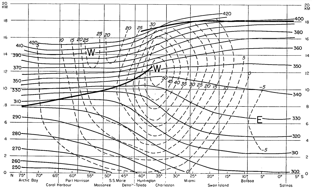
Multiple years of wartime radiosonde temperature soundings at twelve stations near 80^oW, stretching from Salinas, Equador (2^oS) to Coral Harbour (64^oN) and Arctic Bay (74^oN), were used by the American meteorologist Seymour Hess (1948) to construct climatological meridional cross-sections of temperature and geostrophic zonal wind. His result for the geostrophic wind in winter is reproduced here as Figure 2. Most striking is the westerly maximum near 12 km altitude and 35^oN. This showed that, while the tropospheric subtropical jet stream has significant day-to-day variability, it still manifests as a very clear localized wind speed maximum even in a long term mean. Hess apparently felt that poleward of 50oN his data supported plotting the geostrophic wind only up to about 15 or 16 km. With this restricted view one can discern only a hint of vertical shear consistent with a stratospheric high latitude westerly jet.

Also in 1948 Erik Palmén published a similar cross-section based on radiosonde results from stations in Cuba, eastern North America and Greenland.

Henry and Armstrong’s 1949 report on high latitude Canadian observations notes that “the overwhelming majority of the upper wind observations in this report are pilot-balloon ascents. In a few years time when a sufficient quantity of radio-wind data is available, it should be possible to obtain a better picture of wind […] at the higher levels.” Here they reference an important revolution then occurring in the technology of balloon meteorological measurements. The use of steerable directional antennas to track balloon borne radiosondes allowed balloon temperature and pressure data to be obtained up to higher altitudes as well as for the balloon elevation and azimuth to be observed to higher levels (and even during poor visibility conditions). The winds measured in this manner became known as “rawinds” and the measuring system a ”rawinsonde”.

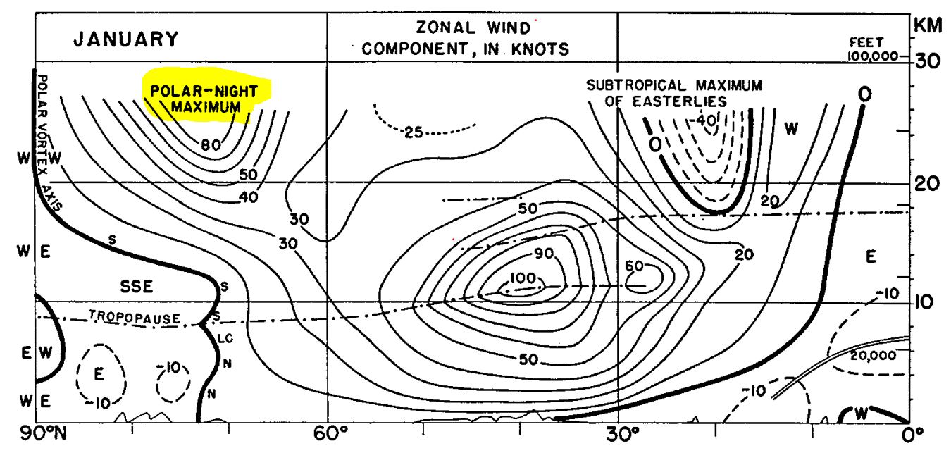
The improved geographical and altitude coverage of the radiosonde network particularly beginning in the late 1940’s allowed the American meteorologist Adam Kochanski (1955) to revisit the 80^oW meridional section using data from 1948-1951. For this period Kochanski notes that data from 17 stations stretching from Panama (9^oN) to Alert (83.5^oN) were available. Kochanski’s result for the January climatology of geostrophic zonal wind is shown here as Figure 3. This represents an improvement over Hess’s earlier results, particularly in the high latitude stratosphere where the climatology is provided up to 30 km and all the way to the pole. Noteworthy was the clear indication of a strong westerly climatological jet peaking at or above 30 km with maximum speed of more than 80 knots ( ~41 m-s^-1). Kochanski referred to this as the “polar-night maximum […] in the middle stratosphere”.

While his high latitude results are fairly realistic, Kochanski’s plot for the tropical and subtropical stratosphere agrees rather poorly with more modern determinations of the zonal wind climatology in the winter hemisphere. Kochanski was at a disadvantage back in 1955, of course, as the equatorial quasibiennial oscillation would not be discovered until 1961.

Using radio wind data

The US military led the development of the technology of radio-tracked weather balloons. Key developments in the late 1940’s were made at the US Army Signal Corps Laboratory in New Jersey. Notably by 1948 they had working versions of the steerable parabolic antenna system later known as GMD-1. Over the next decade GMD-1 would become a standard for most US military and civilian systems and it was confirmed that it produced quite accurate wind determinations. In 1950 C.J. Brasefield of the Signal Corps Laboratory wrote a paper reporting on 20 radiosonde flights using their new technology to measure winds and temperatures up to as high as 35 km at Belmar, New Jersey (42^oN) during July 1948-April 1949. He notes that between ~17 and 35 km the prevailing winds displayed a notable seasonal cycle:

“Between 60,000 ft and 120,000 ft, the winds were easterly during the summer and westerly during the winter. […] Usually the wind speed was still increasing at the bursting altitude of the balloon. These results are consistent with the existence of a stratospheric circumpolar vortex which is cyclonic in winter, anticyclonic in summer. The fragmentary wind data obtained from these flights at high altitudes suggest the possible existence of a stratospheric jet stream in middle latitudes.”

Although Brasefield had very limited data just from just one midlatitude site he successfully intuited key features of the circulation of the extratropical stratosphere, notably suggesting that the circulation might feature a “stratospheric jet stream”.

With a growing network of weather stations featuring radio-tracked rawinsonde measurements, it became practical to characterize the stratospheric circulation using direct wind observations. Warren Godson of the Canadian Meteorological Service and his colleague Roy Lee analysed the Canadian wind observations at high latitudes. They published their results in two important papers: Lee and Godson (1957) and a 1958 paper by Godson and Lee (which is not currently available online) titled “High level fields of wind and temperature over the Canadian Arctic” (volume 31 of the journal Beiträge zur Physik der Atmosphäre).

Lee and Godson (1957) describe their project in their abstract:

“The existence of an Arctic stratospheric jet stream in winter, hitherto largely inferred from mean geostrophic wind sections, is considered on the basis of actual winds for the Canadian Arctic area during the winter of 1955-1956.”

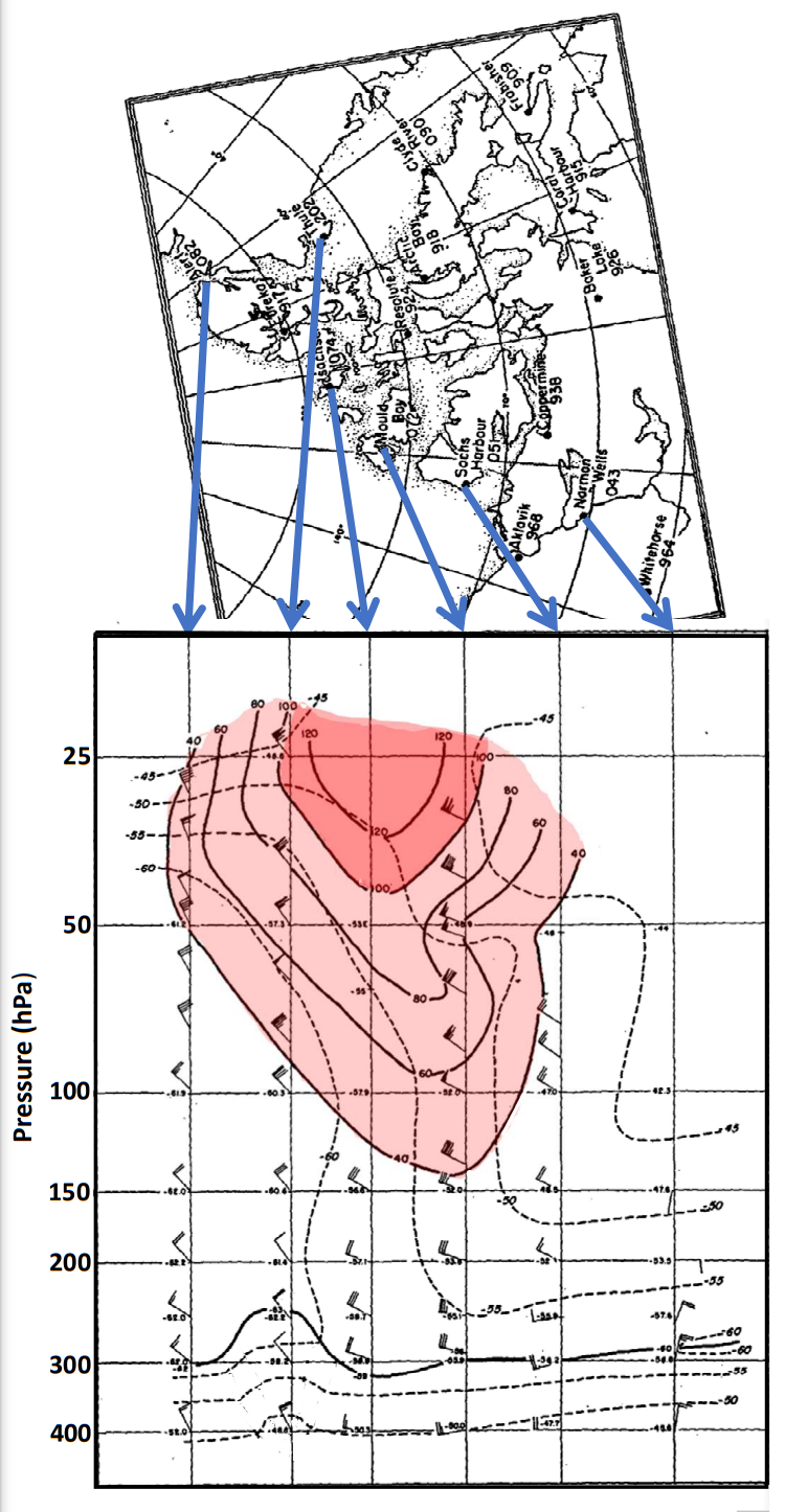
Lee and Godson examined the instantaneous winds on a few selected days during the winter. They noted that the jets that they saw were not aligned exactly zonally and they used the available data to characterize the component of the wind parallel to the jet axis. Figure 4 shows an example from their 1957 paper. The contours are for the north-west component of the wind plotted as a function of distance along the chain of stations shown from Alert (82.5^oN, 62^oW) at the left to Norman Wells (65^oN, 127^oW) on the right, i.e. on a rough northeast-southwest section stretching 2500 km. Here I have combined a map identifying the individual stations with the contour plot of the wind. I have added shading to distinguish regions with north-west winds greater than 40 knots and greater than 100 knots (deep shading). This approach allowed Godson to depict the winds in the core of the jet stream as they appear in an instantaneous snapshot.

In the second paper Godson and Lee (1958) extended their analysis over three winters. They focused on both describing the typical structure of the jet revealed in their data as well as the intraseasonal and interannual variability that is apparent. Quoting their conclusions:

“Vertical cross-sections of the Arctic stratospheric jet stream are presented to show its vertical structure. It is generally found at around 70-75^oN although pronounced meridional movements result in its occurrence as far south as 50^oN. Maximum wind speeds occur above 50 mb and occasionally exceed 230 kt. The rapid-warming epoch in 1957 was the most spectacular at very high levels (Frobisher reported an increase in 25 mb temperature of 34^oC in 24 hours). Vertical time-sections of temperature have revealed major differences in the structure of these warming periods, whose dynamic processes are undoubtedly exceedingly complex”.

The Godson and Lee (1958) paper refers to Richard Scherhag’s pioneering 1952 work on sudden midwinter stratospheric warming which Scherhag saw in Berlin radiosondes, and which he had named the “Berlin phenomenon”. However, Godson and Lee went well beyond Scherhag’s work in characterizing the warmings and the associated changes in the polar vortex. It is noteworthy that the earlier Lee and Godson (1957) paper is cited in a well known and somewhat parallel 1958 analysis of the sudden warming phenomenon by US Weather Bureau scientists Sidney Teweles and Fred Finger.

The papers of Godson and Lee were cited as motivation in several interesting papers that appeared in the next couple of years. Krishnamurti (1959) wrote a paper titled “A vertical cross section through the “polar-night” jet stream” showing a similar analysis as in the Godson papers, but based on data in a 4-day period (December 31, 1957-January 3, 1958) and presenting more detailed analysis, including a plot of the potential vorticity in a section across the jet axis. Palmer (1959) wrote a paper on observations the winter polar stratospheric vortex including a comparison of the situation in the Arctic and Antarctic. The question of whether the polar night jet is baroclinically unstable was addressed by Murray (1960), and Murray’s paper helped inspire one of the all-time most famous papers in the field of geophysical fluid dynamics, namely the study of the necessary conditions for baroclinic instability by Charney and Stern (1962).

Blooming Interest in Polar Stratosphere Research

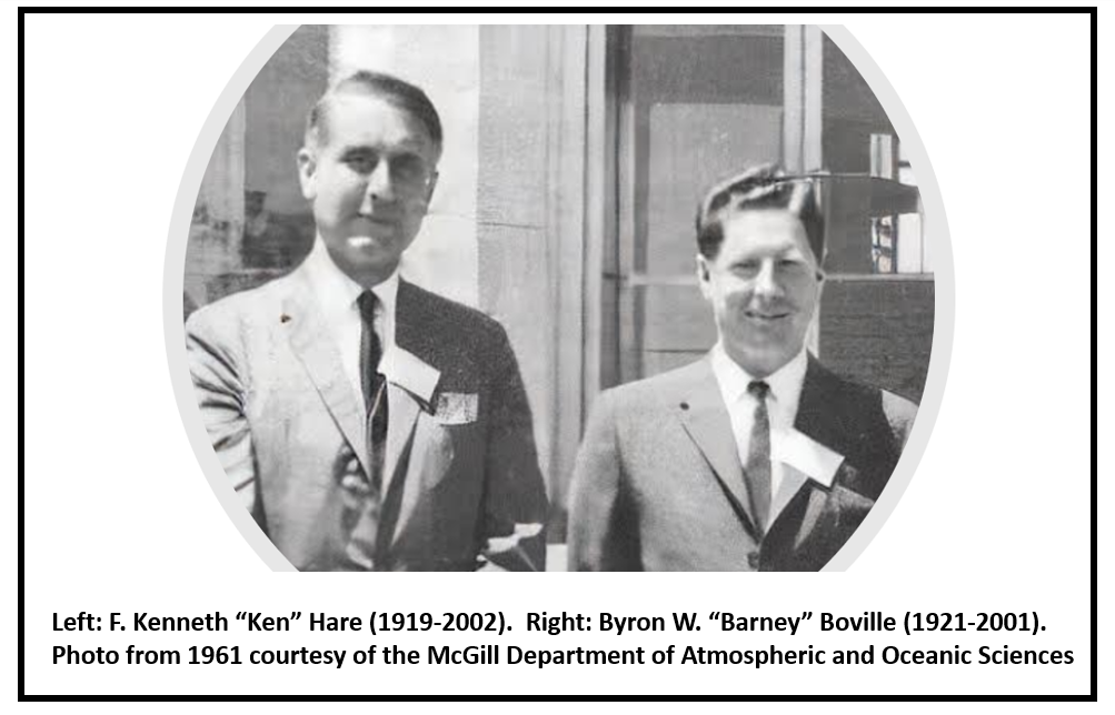
The initial papers on the polar night jet opened an era of enhanced interest in the dynamics of the polar stratosphere and Canadian scientists and institutions would take the lead. Notably McGill University’s researchers led by professors Ken Hare and Byron W. Boville would continue with observational studies of the circulation in the polar stratosphere. McGill’s biennial “Stanstead Seminar” series, founded by Hare in 1955, would become a leading venue for discussing developments in stratospheric research. The was titled “The Stratosphere and Mesosphere and Polar Meteorology” and attracted an international group of outstanding researchers. The 1965 Stanstead Seminar was titled “The Middle Atmosphere”. Hare’s introduction to the 1963 proceedings volume included his perspective on recent history:

“In 1959 when we first devoted the Seminar in part to stratospheric questions, research at such levels was something of a novelty. The McGill group felt itself to be among pioneers. Four years later all is changed. Stratospheric and mesospheric problems occupy the centre of the stage.”

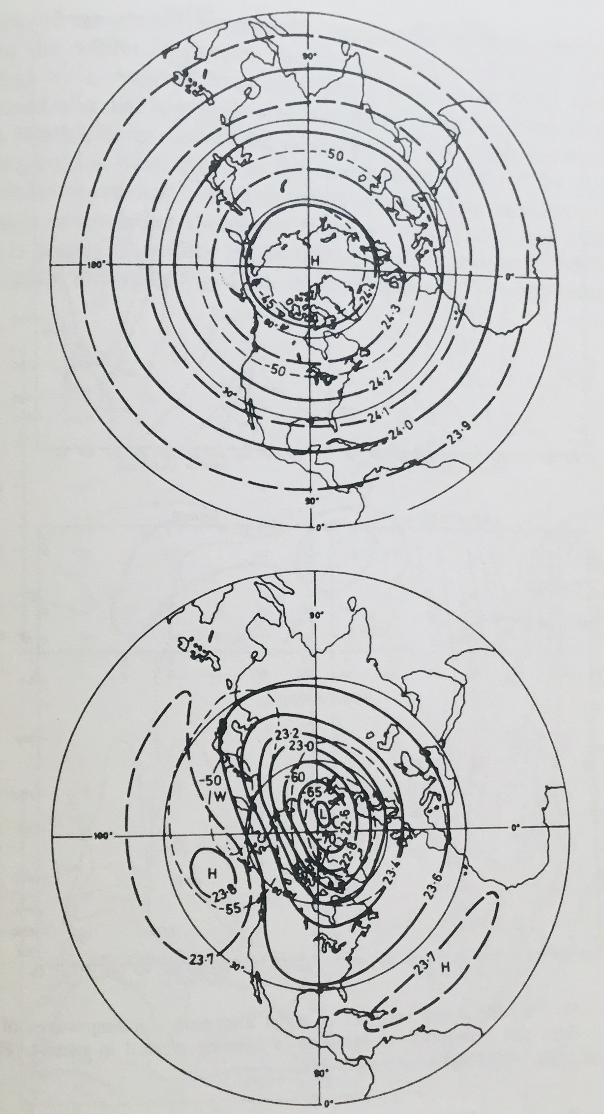
The research at McGill in the early 1960’s would provide important empirical input into seminal work on stratospheric dynamics over the subsequent decade. I will mention here two notable examples. First the classic 1970 paper of Taroh Matsuno formulating a numerical model of stationary Rossby waves in the extratropical stratosphere includes as motivation references to three of Boville’s observational papers (1960, 1963, 1966). In 1971 Matsuno generalized his 1970 model and made the fundamental discovery of the mechanism of stratospheric sudden warmings. Then Jim Holton in his 1975 pioneering monograph The Dynamic Meteorology of the Stratosphere and Mesosphere includes a version of a figure prepared by Hare showing a polar projection of the long term mean January and July 30 hPa heights (reproduced here as Figure 5). This served as the fundamental observational background to Holton’s discussion of stratospheric quasi-stationary Rossby waves.

The term “Polar Night Jet (Stream)”

It is difficult to identify a precise moment of discovery for the stratospheric polar night jet stream phenomenon. But what about the name “polar night jet/polar night jet stream”? My survey of the literature shows that the term was probably unknown before about 1957 but quickly became popular, so that by 1960 it had become a standard piece of meteorological nomenclature and had even appeared in the popular media. As noted earlier, the two key pioneering papers of 1955-1957 did not use the term: Kochanski (1955) referring to a “polar night maximum” and Lee and Godson (1957) referring to the “Arctic stratospheric jet stream”. Krishnamurti (1959) may be the first journal article with “polar-night jet stream” in the title.

Remarkably, the newly discovered phenomenon was referred to in an article meant for the general public in the April 1958 issue of Popular Mechanics. The article discussed recent developments in weather forecasting and mainly focused on tropospheric jet streams. However it also notes that “the most recently discovered planetary wind band, dubbed the polar night jet, flows around earth 80,000 feet above the Arctic circle” and even displayed a schematic diagram of the Northern Hemisphere atmosphere including a depiction of the polar night jet.

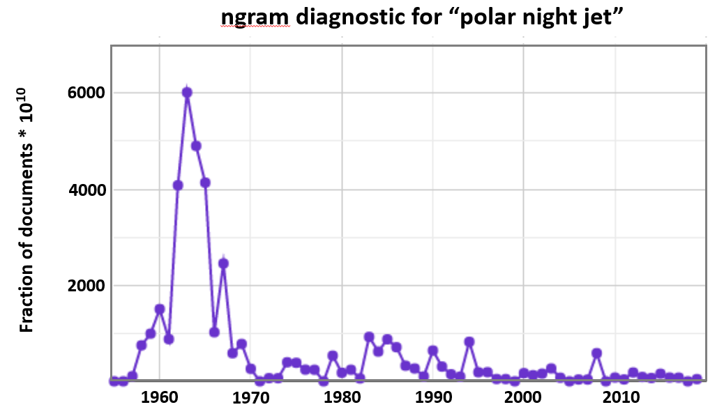
I evaluated the evolving popularity of the term “polar night jet (stream)” using the google “ngram viewer” application. The ngram and its application to studying the history of science is described in more detail here. The ngram viewer analyzes the entirety of the digitized documents available to Google Books and determines the frequency of use for any given phrase in individual calendar years. Specifically ngram produces a measure of the ratio of pages containing the phrase to the total number of pages of text available in that year. Figure 6 shows the yearly ngram measures for the phrase “polar night jet”. The ngram viewer results are known to have issues with errors in the optical character recognition procedures and with misdating of documents – and so the results can be noisy. In any event Fig. 6 shows vividly the growth in popularity of the concept of the polar -night jet in the late 1950’s and early 1960’s.

To the Present Day

The term “polar night jet” or “polar night jet stream” is still widely used and is introduced to students in today’s standard textbook of stratospheric meteorology. The term may seem slightly dated or potentially misleading for some students, however, as it may suggest a jet that is anchored to the edge of the polar night, while the real jet is, of course, much more dynamic. Indeed the declining word count (Fig. 6) may reflect a modern tendency to consider the stratospheric polar vortex as a whole as a region of high potential vorticity, rather than focusing on the jet-like wind maximum. However, the term “polar night jet” is still quite evocative – one readily imagines a ring of powerful winds streaming high above the ground in the polar darkness – and in 2020 it even inspired an electronic music composition by the Estonian musician Lauri-Dag Tüür.

Kevin Hamilton is Emeritus Professor of Atmospheric Sciences and retired Director of the International Pacific Research Center (IPRC) at the University of Hawaii. He has had a long career in academia and government including stints at McGill and the University of British Columbia in the 1980’s. His main research interests have been in stratospheric dynamics and climate modeling, but he has also investigated aspects of the history of meteorology. He currently serves as an Editor of the journal History of Geo- and Space Sciences.